library(tidyverse)
library(gt)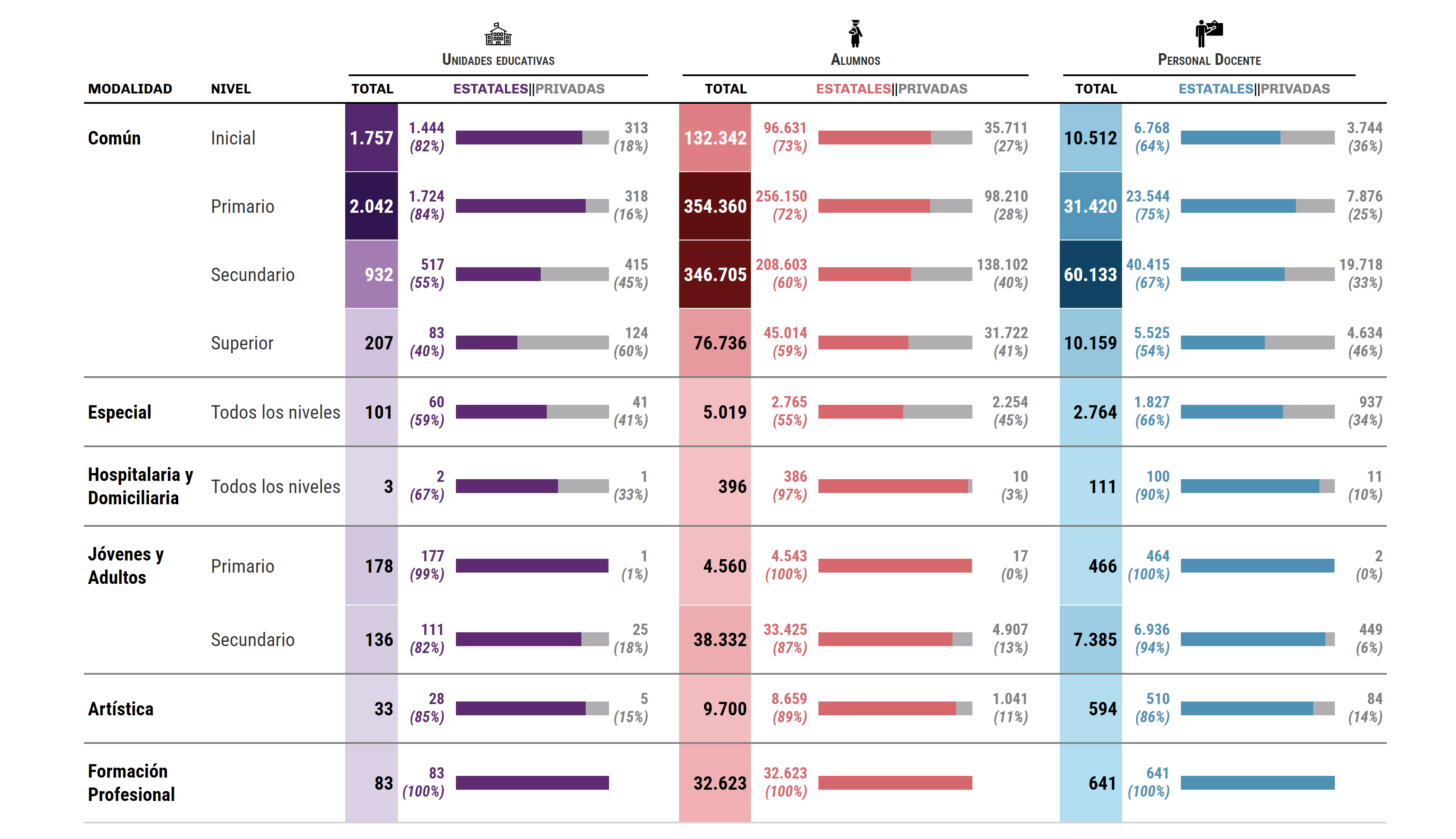
library(gtExtras)En este post veremos un paso a paso de cómo generar una tabla “con estilo” ✨ usando las librerias gt y gtExtra. Esta tabla la diseñé para una infografía que resumen y muestra datos del sistema educativo en Córdoba Capital en el 2023 y acompaña a otras visualizaciones que no se verán en esta mini guía.
Librerias utilizadas
Cargamos las librerias necesarias, en este caso usaremos solamente las siguientes:
Datos
Usaremos datos provenientes del relevamiento anual para establecimientos educativos de la provincia de Córdoba, procesados previamente (por mí) y disponibles para descargar en .csv:
data <- read_csv("data/datos_se_2023.csv")

data
# A tibble: 10 × 11
Modalidad Nivel UE_Total UE_Estatal UE_Privado ALUM_Total ALUM_Estatal
<chr> <chr> <dbl> <dbl> <dbl> <dbl> <dbl>
1 Común Inic… 1757 1444 313 132342 96631
2 Común Prim… 2042 1724 318 354360 256150
3 Común Secu… 932 517 415 346705 208603
4 Común Supe… 207 83 124 76736 45014
5 Especial Todo… 101 60 41 5019 2765
6 Hospitalaria y … Todo… 3 2 1 396 386
7 Jóvenes y Adult… Prim… 178 177 1 4560 4543
8 Jóvenes y Adult… Secu… 136 111 25 38332 33425
9 Artística <NA> 33 28 5 9700 8659
10 Formación Profe… <NA> 83 83 0 32623 32623
# ℹ 4 more variables: ALUM_Privado <dbl>, PD_Total <dbl>, PD_Estatal <dbl>,
# PD_Privado <dbl>Objetivo
El objetivo será generar la siguiente tabla
Construcción de tabla
Antes de arrancar vamos a definir algunos valores constantes.
img_height <- 32

div_total_pct_text <- "<div style='line-height:21px'>"
El primer paso será agregar algunas columnas, limpiar o corregir otras:
tabla1 <- data |>
mutate(Nivel = case_when(
is.na(Nivel) ~ "",
TRUE ~ Nivel
)) |>
mutate(
UE_Estatal = as.numeric(UE_Estatal)
) |>
mutate(
Modalidad = case_when(
Modalidad == "Hospitalaria y Domiciliaria" ~ "Hospitalaria y <br>Domiciliaria",
Modalidad == "Jóvenes y Adultos" ~ "Jóvenes y<br>Adultos",
Modalidad == "Formación Profesional" ~ "Formación<br>Profesional",
TRUE ~ Modalidad
)
) |>
rowwise() |>
mutate(
#percents_ue = pmap(list(UE_Estatal,UE_Privado,UE_Total), ~c((..1/..3),(..2/..3))),
percents_ue = UE_Estatal/UE_Total,
percents_ue2 = UE_Privado/UE_Total,
UE_Estatal = if_else(UE_Estatal > 0,
str_c(div_total_pct_text, scales::label_comma(big.mark = ".", accuracy = 1)(UE_Estatal),"<br><i>(",scales::label_percent()(percents_ue),")</i></div>"), ""),
UE_Privado = if_else(UE_Privado > 0, str_c(div_total_pct_text, scales::label_comma(big.mark = ".", accuracy = 1)(UE_Privado),"<br><i>(",scales::label_percent()(percents_ue2),")</i></div>"), ""),
#percents_alu = pmap(list(ALUM_Estatal,ALUM_Privado,ALUM_Total), ~c((..1/..3),(..2/..3))),
percents_alu = ALUM_Estatal/ALUM_Total,
percents_alu2 = ALUM_Privado/ALUM_Total,
ALUM_Estatal = if_else(ALUM_Estatal > 0,
str_c(div_total_pct_text, scales::label_comma(big.mark = ".", accuracy = 1)(ALUM_Estatal),"<br><i>(",scales::label_percent()(percents_alu),")</i></div>"), ""),
ALUM_Privado = if_else(ALUM_Privado > 0,
str_c(div_total_pct_text, scales::label_comma(big.mark = ".", accuracy = 1)(ALUM_Privado),"<br><i>(",scales::label_percent()(percents_alu2),")</i></div>"), ""),
#percents_pd = pmap(list(PD_Estatal,PD_Privado,PD_Total), ~c((..1/..3),(..2/..3)))
percents_pd = PD_Estatal/PD_Total,
percents_pd2 = PD_Privado/PD_Total,
PD_Estatal = if_else(PD_Estatal > 0,
str_c(div_total_pct_text, scales::label_comma(big.mark = ".", accuracy = 1)(PD_Estatal),"<br><i>(",scales::label_percent()(percents_pd),")</i></div>"), ""),
PD_Privado = if_else(PD_Privado > 0,
str_c(div_total_pct_text, scales::label_comma(big.mark = ".", accuracy = 1)(PD_Privado),"<br><i>(",scales::label_percent()(percents_pd2),")</i></div>"), "")
) |>
gt(id = "tabla")
tabla1| Modalidad | Nivel | UE_Total | UE_Estatal | UE_Privado | ALUM_Total | ALUM_Estatal | ALUM_Privado | PD_Total | PD_Estatal | PD_Privado | percents_ue | percents_ue2 | percents_alu | percents_alu2 | percents_pd | percents_pd2 |
|---|---|---|---|---|---|---|---|---|---|---|---|---|---|---|---|---|
| Común | Inicial | 1757 | <div style='line-height:21px'>1.444<br><i>(82%)</i></div> | <div style='line-height:21px'>313<br><i>(18%)</i></div> | 132342 | <div style='line-height:21px'>96.631<br><i>(73%)</i></div> | <div style='line-height:21px'>35.711<br><i>(27%)</i></div> | 10512 | <div style='line-height:21px'>6.768<br><i>(64%)</i></div> | <div style='line-height:21px'>3.744<br><i>(36%)</i></div> | 0.8218554 | 0.178144565 | 0.7301612 | 0.26983875 | 0.6438356 | 0.356164384 |
| Común | Primario | 2042 | <div style='line-height:21px'>1.724<br><i>(84%)</i></div> | <div style='line-height:21px'>318<br><i>(16%)</i></div> | 354360 | <div style='line-height:21px'>256.150<br><i>(72%)</i></div> | <div style='line-height:21px'>98.210<br><i>(28%)</i></div> | 31420 | <div style='line-height:21px'>23.544<br><i>(75%)</i></div> | <div style='line-height:21px'>7.876<br><i>(25%)</i></div> | 0.8442703 | 0.155729677 | 0.7228525 | 0.27714753 | 0.7493316 | 0.250668364 |
| Común | Secundario | 932 | <div style='line-height:21px'>517<br><i>(55%)</i></div> | <div style='line-height:21px'>415<br><i>(45%)</i></div> | 346705 | <div style='line-height:21px'>208.603<br><i>(60%)</i></div> | <div style='line-height:21px'>138.102<br><i>(40%)</i></div> | 60133 | <div style='line-height:21px'>40.415<br><i>(67%)</i></div> | <div style='line-height:21px'>19.718<br><i>(33%)</i></div> | 0.5547210 | 0.445278970 | 0.6016729 | 0.39832711 | 0.6720935 | 0.327906474 |
| Común | Superior | 207 | <div style='line-height:21px'>83<br><i>(40%)</i></div> | <div style='line-height:21px'>124<br><i>(60%)</i></div> | 76736 | <div style='line-height:21px'>45.014<br><i>(59%)</i></div> | <div style='line-height:21px'>31.722<br><i>(41%)</i></div> | 10159 | <div style='line-height:21px'>5.525<br><i>(54%)</i></div> | <div style='line-height:21px'>4.634<br><i>(46%)</i></div> | 0.4009662 | 0.599033816 | 0.5866086 | 0.41339137 | 0.5438527 | 0.456147259 |
| Especial | Todos los niveles | 101 | <div style='line-height:21px'>60<br><i>(59%)</i></div> | <div style='line-height:21px'>41<br><i>(41%)</i></div> | 5019 | <div style='line-height:21px'>2.765<br><i>(55%)</i></div> | <div style='line-height:21px'>2.254<br><i>(45%)</i></div> | 2764 | <div style='line-height:21px'>1.827<br><i>(66%)</i></div> | <div style='line-height:21px'>937<br><i>(34%)</i></div> | 0.5940594 | 0.405940594 | 0.5509066 | 0.44909344 | 0.6609986 | 0.339001447 |
| Hospitalaria y <br>Domiciliaria | Todos los niveles | 3 | <div style='line-height:21px'>2<br><i>(67%)</i></div> | <div style='line-height:21px'>1<br><i>(33%)</i></div> | 396 | <div style='line-height:21px'>386<br><i>(97%)</i></div> | <div style='line-height:21px'>10<br><i>(3%)</i></div> | 111 | <div style='line-height:21px'>100<br><i>(90%)</i></div> | <div style='line-height:21px'>11<br><i>(10%)</i></div> | 0.6666667 | 0.333333333 | 0.9747475 | 0.02525253 | 0.9009009 | 0.099099099 |
| Jóvenes y<br>Adultos | Primario | 178 | <div style='line-height:21px'>177<br><i>(99%)</i></div> | <div style='line-height:21px'>1<br><i>(1%)</i></div> | 4560 | <div style='line-height:21px'>4.543<br><i>(100%)</i></div> | <div style='line-height:21px'>17<br><i>(0%)</i></div> | 466 | <div style='line-height:21px'>464<br><i>(100%)</i></div> | <div style='line-height:21px'>2<br><i>(0%)</i></div> | 0.9943820 | 0.005617978 | 0.9962719 | 0.00372807 | 0.9957082 | 0.004291845 |
| Jóvenes y<br>Adultos | Secundario | 136 | <div style='line-height:21px'>111<br><i>(82%)</i></div> | <div style='line-height:21px'>25<br><i>(18%)</i></div> | 38332 | <div style='line-height:21px'>33.425<br><i>(87%)</i></div> | <div style='line-height:21px'>4.907<br><i>(13%)</i></div> | 7385 | <div style='line-height:21px'>6.936<br><i>(94%)</i></div> | <div style='line-height:21px'>449<br><i>(6%)</i></div> | 0.8161765 | 0.183823529 | 0.8719869 | 0.12801315 | 0.9392011 | 0.060798917 |
| Artística | 33 | <div style='line-height:21px'>28<br><i>(85%)</i></div> | <div style='line-height:21px'>5<br><i>(15%)</i></div> | 9700 | <div style='line-height:21px'>8.659<br><i>(89%)</i></div> | <div style='line-height:21px'>1.041<br><i>(11%)</i></div> | 594 | <div style='line-height:21px'>510<br><i>(86%)</i></div> | <div style='line-height:21px'>84<br><i>(14%)</i></div> | 0.8484848 | 0.151515152 | 0.8926804 | 0.10731959 | 0.8585859 | 0.141414141 | |
| Formación<br>Profesional | 83 | <div style='line-height:21px'>83<br><i>(100%)</i></div> | 32623 | <div style='line-height:21px'>32.623<br><i>(100%)</i></div> | 641 | <div style='line-height:21px'>641<br><i>(100%)</i></div> | 1.0000000 | 0.000000000 | 1.0000000 | 0.00000000 | 1.0000000 | 0.000000000 |
Agregamos un tema predefinido a la tabla, en este caso el famoso FiveThirtyEight. Este tema servirá como base.
tabla2 <- tabla1 |>
  gt_theme_538()

tabla2| Modalidad | Nivel | UE_Total | UE_Estatal | UE_Privado | ALUM_Total | ALUM_Estatal | ALUM_Privado | PD_Total | PD_Estatal | PD_Privado | percents_ue | percents_ue2 | percents_alu | percents_alu2 | percents_pd | percents_pd2 |
|---|---|---|---|---|---|---|---|---|---|---|---|---|---|---|---|---|
| Común | Inicial | 1757 | <div style='line-height:21px'>1.444<br><i>(82%)</i></div> | <div style='line-height:21px'>313<br><i>(18%)</i></div> | 132342 | <div style='line-height:21px'>96.631<br><i>(73%)</i></div> | <div style='line-height:21px'>35.711<br><i>(27%)</i></div> | 10512 | <div style='line-height:21px'>6.768<br><i>(64%)</i></div> | <div style='line-height:21px'>3.744<br><i>(36%)</i></div> | 0.8218554 | 0.178144565 | 0.7301612 | 0.26983875 | 0.6438356 | 0.356164384 |
| Común | Primario | 2042 | <div style='line-height:21px'>1.724<br><i>(84%)</i></div> | <div style='line-height:21px'>318<br><i>(16%)</i></div> | 354360 | <div style='line-height:21px'>256.150<br><i>(72%)</i></div> | <div style='line-height:21px'>98.210<br><i>(28%)</i></div> | 31420 | <div style='line-height:21px'>23.544<br><i>(75%)</i></div> | <div style='line-height:21px'>7.876<br><i>(25%)</i></div> | 0.8442703 | 0.155729677 | 0.7228525 | 0.27714753 | 0.7493316 | 0.250668364 |
| Común | Secundario | 932 | <div style='line-height:21px'>517<br><i>(55%)</i></div> | <div style='line-height:21px'>415<br><i>(45%)</i></div> | 346705 | <div style='line-height:21px'>208.603<br><i>(60%)</i></div> | <div style='line-height:21px'>138.102<br><i>(40%)</i></div> | 60133 | <div style='line-height:21px'>40.415<br><i>(67%)</i></div> | <div style='line-height:21px'>19.718<br><i>(33%)</i></div> | 0.5547210 | 0.445278970 | 0.6016729 | 0.39832711 | 0.6720935 | 0.327906474 |
| Común | Superior | 207 | <div style='line-height:21px'>83<br><i>(40%)</i></div> | <div style='line-height:21px'>124<br><i>(60%)</i></div> | 76736 | <div style='line-height:21px'>45.014<br><i>(59%)</i></div> | <div style='line-height:21px'>31.722<br><i>(41%)</i></div> | 10159 | <div style='line-height:21px'>5.525<br><i>(54%)</i></div> | <div style='line-height:21px'>4.634<br><i>(46%)</i></div> | 0.4009662 | 0.599033816 | 0.5866086 | 0.41339137 | 0.5438527 | 0.456147259 |
| Especial | Todos los niveles | 101 | <div style='line-height:21px'>60<br><i>(59%)</i></div> | <div style='line-height:21px'>41<br><i>(41%)</i></div> | 5019 | <div style='line-height:21px'>2.765<br><i>(55%)</i></div> | <div style='line-height:21px'>2.254<br><i>(45%)</i></div> | 2764 | <div style='line-height:21px'>1.827<br><i>(66%)</i></div> | <div style='line-height:21px'>937<br><i>(34%)</i></div> | 0.5940594 | 0.405940594 | 0.5509066 | 0.44909344 | 0.6609986 | 0.339001447 |
| Hospitalaria y <br>Domiciliaria | Todos los niveles | 3 | <div style='line-height:21px'>2<br><i>(67%)</i></div> | <div style='line-height:21px'>1<br><i>(33%)</i></div> | 396 | <div style='line-height:21px'>386<br><i>(97%)</i></div> | <div style='line-height:21px'>10<br><i>(3%)</i></div> | 111 | <div style='line-height:21px'>100<br><i>(90%)</i></div> | <div style='line-height:21px'>11<br><i>(10%)</i></div> | 0.6666667 | 0.333333333 | 0.9747475 | 0.02525253 | 0.9009009 | 0.099099099 |
| Jóvenes y<br>Adultos | Primario | 178 | <div style='line-height:21px'>177<br><i>(99%)</i></div> | <div style='line-height:21px'>1<br><i>(1%)</i></div> | 4560 | <div style='line-height:21px'>4.543<br><i>(100%)</i></div> | <div style='line-height:21px'>17<br><i>(0%)</i></div> | 466 | <div style='line-height:21px'>464<br><i>(100%)</i></div> | <div style='line-height:21px'>2<br><i>(0%)</i></div> | 0.9943820 | 0.005617978 | 0.9962719 | 0.00372807 | 0.9957082 | 0.004291845 |
| Jóvenes y<br>Adultos | Secundario | 136 | <div style='line-height:21px'>111<br><i>(82%)</i></div> | <div style='line-height:21px'>25<br><i>(18%)</i></div> | 38332 | <div style='line-height:21px'>33.425<br><i>(87%)</i></div> | <div style='line-height:21px'>4.907<br><i>(13%)</i></div> | 7385 | <div style='line-height:21px'>6.936<br><i>(94%)</i></div> | <div style='line-height:21px'>449<br><i>(6%)</i></div> | 0.8161765 | 0.183823529 | 0.8719869 | 0.12801315 | 0.9392011 | 0.060798917 |
| Artística | 33 | <div style='line-height:21px'>28<br><i>(85%)</i></div> | <div style='line-height:21px'>5<br><i>(15%)</i></div> | 9700 | <div style='line-height:21px'>8.659<br><i>(89%)</i></div> | <div style='line-height:21px'>1.041<br><i>(11%)</i></div> | 594 | <div style='line-height:21px'>510<br><i>(86%)</i></div> | <div style='line-height:21px'>84<br><i>(14%)</i></div> | 0.8484848 | 0.151515152 | 0.8926804 | 0.10731959 | 0.8585859 | 0.141414141 | |
| Formación<br>Profesional | 83 | <div style='line-height:21px'>83<br><i>(100%)</i></div> | 32623 | <div style='line-height:21px'>32.623<br><i>(100%)</i></div> | 641 | <div style='line-height:21px'>641<br><i>(100%)</i></div> | 1.0000000 | 0.000000000 | 1.0000000 | 0.00000000 | 1.0000000 | 0.000000000 |
Ahora agregaremos las columnas que tienen la barra porcentual indicando la distribución de totales por tipo de gestión (estatal o privada). Cabe destacar que utilizaremos un esquema de colores que permita diferenciar cada dimensión: Unidades Educativas, Alumnos y Personal Docente.
tabla3 <- tabla2 |>
  # Creamos barras de porcentaje
  gt_plt_bar_pct(column = percents_ue, fill = "#5e2a72", background = "#B0AEB0")  |>
  gt_plt_bar_pct(column = percents_alu, fill = "#d5676d", background = "#B0AEB0")  |>
  gt_plt_bar_pct(column = percents_pd, fill = "#4f91b4", background = "#B0AEB0")  |>

  # Ocultamos algunas columnas
  cols_hide(
    columns = c(percents_ue2, percents_alu2, percents_pd2)
  )

tabla3| Modalidad | Nivel | UE_Total | UE_Estatal | UE_Privado | ALUM_Total | ALUM_Estatal | ALUM_Privado | PD_Total | PD_Estatal | PD_Privado | percents_ue | percents_alu | percents_pd |
|---|---|---|---|---|---|---|---|---|---|---|---|---|---|
| Común | Inicial | 1757 | <div style='line-height:21px'>1.444<br><i>(82%)</i></div> | <div style='line-height:21px'>313<br><i>(18%)</i></div> | 132342 | <div style='line-height:21px'>96.631<br><i>(73%)</i></div> | <div style='line-height:21px'>35.711<br><i>(27%)</i></div> | 10512 | <div style='line-height:21px'>6.768<br><i>(64%)</i></div> | <div style='line-height:21px'>3.744<br><i>(36%)</i></div> | |||
| Común | Primario | 2042 | <div style='line-height:21px'>1.724<br><i>(84%)</i></div> | <div style='line-height:21px'>318<br><i>(16%)</i></div> | 354360 | <div style='line-height:21px'>256.150<br><i>(72%)</i></div> | <div style='line-height:21px'>98.210<br><i>(28%)</i></div> | 31420 | <div style='line-height:21px'>23.544<br><i>(75%)</i></div> | <div style='line-height:21px'>7.876<br><i>(25%)</i></div> | |||
| Común | Secundario | 932 | <div style='line-height:21px'>517<br><i>(55%)</i></div> | <div style='line-height:21px'>415<br><i>(45%)</i></div> | 346705 | <div style='line-height:21px'>208.603<br><i>(60%)</i></div> | <div style='line-height:21px'>138.102<br><i>(40%)</i></div> | 60133 | <div style='line-height:21px'>40.415<br><i>(67%)</i></div> | <div style='line-height:21px'>19.718<br><i>(33%)</i></div> | |||
| Común | Superior | 207 | <div style='line-height:21px'>83<br><i>(40%)</i></div> | <div style='line-height:21px'>124<br><i>(60%)</i></div> | 76736 | <div style='line-height:21px'>45.014<br><i>(59%)</i></div> | <div style='line-height:21px'>31.722<br><i>(41%)</i></div> | 10159 | <div style='line-height:21px'>5.525<br><i>(54%)</i></div> | <div style='line-height:21px'>4.634<br><i>(46%)</i></div> | |||
| Especial | Todos los niveles | 101 | <div style='line-height:21px'>60<br><i>(59%)</i></div> | <div style='line-height:21px'>41<br><i>(41%)</i></div> | 5019 | <div style='line-height:21px'>2.765<br><i>(55%)</i></div> | <div style='line-height:21px'>2.254<br><i>(45%)</i></div> | 2764 | <div style='line-height:21px'>1.827<br><i>(66%)</i></div> | <div style='line-height:21px'>937<br><i>(34%)</i></div> | |||
| Hospitalaria y <br>Domiciliaria | Todos los niveles | 3 | <div style='line-height:21px'>2<br><i>(67%)</i></div> | <div style='line-height:21px'>1<br><i>(33%)</i></div> | 396 | <div style='line-height:21px'>386<br><i>(97%)</i></div> | <div style='line-height:21px'>10<br><i>(3%)</i></div> | 111 | <div style='line-height:21px'>100<br><i>(90%)</i></div> | <div style='line-height:21px'>11<br><i>(10%)</i></div> | |||
| Jóvenes y<br>Adultos | Primario | 178 | <div style='line-height:21px'>177<br><i>(99%)</i></div> | <div style='line-height:21px'>1<br><i>(1%)</i></div> | 4560 | <div style='line-height:21px'>4.543<br><i>(100%)</i></div> | <div style='line-height:21px'>17<br><i>(0%)</i></div> | 466 | <div style='line-height:21px'>464<br><i>(100%)</i></div> | <div style='line-height:21px'>2<br><i>(0%)</i></div> | |||
| Jóvenes y<br>Adultos | Secundario | 136 | <div style='line-height:21px'>111<br><i>(82%)</i></div> | <div style='line-height:21px'>25<br><i>(18%)</i></div> | 38332 | <div style='line-height:21px'>33.425<br><i>(87%)</i></div> | <div style='line-height:21px'>4.907<br><i>(13%)</i></div> | 7385 | <div style='line-height:21px'>6.936<br><i>(94%)</i></div> | <div style='line-height:21px'>449<br><i>(6%)</i></div> | |||
| Artística | 33 | <div style='line-height:21px'>28<br><i>(85%)</i></div> | <div style='line-height:21px'>5<br><i>(15%)</i></div> | 9700 | <div style='line-height:21px'>8.659<br><i>(89%)</i></div> | <div style='line-height:21px'>1.041<br><i>(11%)</i></div> | 594 | <div style='line-height:21px'>510<br><i>(86%)</i></div> | <div style='line-height:21px'>84<br><i>(14%)</i></div> | ||||
| Formación<br>Profesional | 83 | <div style='line-height:21px'>83<br><i>(100%)</i></div> | 32623 | <div style='line-height:21px'>32.623<br><i>(100%)</i></div> | 641 | <div style='line-height:21px'>641<br><i>(100%)</i></div> |
Además de los colores, agregaremos los spanners o agrupaciones de columnas que permitirán identificar rápidamente los datos que pertenecen a cada dimensión:
tabla4_spanner <- tabla3 |>
  # Conf. Spanner para Instituciones
  tab_spanner(
    label = md(
      paste(
        local_image("imgs/school-building-with-flag-svgrepo-com.svg", height = img_height),
        "<div style='line-height:25px'><span style='font-weight:bold;font-variant:small-caps;font-size:19px'>Unidades educativas</div>"
        )
      ),
    columns = c("UE_Total","UE_Estatal","percents_ue","UE_Privado"),
    id = "ue"
  )  |>
  # Conf. Spanner para Alumnos
  tab_spanner(
    label = md(
      paste(
        local_image("imgs/student-svgrepo-com.svg", height = img_height),
        "<div style='line-height:25px'><span style='font-weight:bold;font-variant:small-caps;font-size:19px'>Alumnos</div>"
      )
    ),
    columns = c("ALUM_Total","ALUM_Estatal","percents_alu","ALUM_Privado"),
    id = "alumnos"
  )  |>
  # Conf. Spanner para Personal Docente
  tab_spanner(
    label = md(
      paste(
        local_image("imgs/teacher-svgrepo-com.svg", height = img_height),
        "<div style='line-height:25px'><span style='font-weight:bold;font-variant:small-caps;font-size:19px;'>Personal Docente</div>"
      )
    ),
    columns = c("PD_Total","PD_Estatal","percents_pd","PD_Privado"),
    id = "pd"
  )

tabla4_spanner| Modalidad | Nivel |
 Unidades educativas
|
 Alumnos
|
 Personal Docente
|
|||||||||
|---|---|---|---|---|---|---|---|---|---|---|---|---|---|
| UE_Total | UE_Estatal | percents_ue | UE_Privado | ALUM_Total | ALUM_Estatal | percents_alu | ALUM_Privado | PD_Total | PD_Estatal | percents_pd | PD_Privado | ||
| Común | Inicial | 1757 | <div style='line-height:21px'>1.444<br><i>(82%)</i></div> | <div style='line-height:21px'>313<br><i>(18%)</i></div> | 132342 | <div style='line-height:21px'>96.631<br><i>(73%)</i></div> | <div style='line-height:21px'>35.711<br><i>(27%)</i></div> | 10512 | <div style='line-height:21px'>6.768<br><i>(64%)</i></div> | <div style='line-height:21px'>3.744<br><i>(36%)</i></div> | |||
| Común | Primario | 2042 | <div style='line-height:21px'>1.724<br><i>(84%)</i></div> | <div style='line-height:21px'>318<br><i>(16%)</i></div> | 354360 | <div style='line-height:21px'>256.150<br><i>(72%)</i></div> | <div style='line-height:21px'>98.210<br><i>(28%)</i></div> | 31420 | <div style='line-height:21px'>23.544<br><i>(75%)</i></div> | <div style='line-height:21px'>7.876<br><i>(25%)</i></div> | |||
| Común | Secundario | 932 | <div style='line-height:21px'>517<br><i>(55%)</i></div> | <div style='line-height:21px'>415<br><i>(45%)</i></div> | 346705 | <div style='line-height:21px'>208.603<br><i>(60%)</i></div> | <div style='line-height:21px'>138.102<br><i>(40%)</i></div> | 60133 | <div style='line-height:21px'>40.415<br><i>(67%)</i></div> | <div style='line-height:21px'>19.718<br><i>(33%)</i></div> | |||
| Común | Superior | 207 | <div style='line-height:21px'>83<br><i>(40%)</i></div> | <div style='line-height:21px'>124<br><i>(60%)</i></div> | 76736 | <div style='line-height:21px'>45.014<br><i>(59%)</i></div> | <div style='line-height:21px'>31.722<br><i>(41%)</i></div> | 10159 | <div style='line-height:21px'>5.525<br><i>(54%)</i></div> | <div style='line-height:21px'>4.634<br><i>(46%)</i></div> | |||
| Especial | Todos los niveles | 101 | <div style='line-height:21px'>60<br><i>(59%)</i></div> | <div style='line-height:21px'>41<br><i>(41%)</i></div> | 5019 | <div style='line-height:21px'>2.765<br><i>(55%)</i></div> | <div style='line-height:21px'>2.254<br><i>(45%)</i></div> | 2764 | <div style='line-height:21px'>1.827<br><i>(66%)</i></div> | <div style='line-height:21px'>937<br><i>(34%)</i></div> | |||
| Hospitalaria y <br>Domiciliaria | Todos los niveles | 3 | <div style='line-height:21px'>2<br><i>(67%)</i></div> | <div style='line-height:21px'>1<br><i>(33%)</i></div> | 396 | <div style='line-height:21px'>386<br><i>(97%)</i></div> | <div style='line-height:21px'>10<br><i>(3%)</i></div> | 111 | <div style='line-height:21px'>100<br><i>(90%)</i></div> | <div style='line-height:21px'>11<br><i>(10%)</i></div> | |||
| Jóvenes y<br>Adultos | Primario | 178 | <div style='line-height:21px'>177<br><i>(99%)</i></div> | <div style='line-height:21px'>1<br><i>(1%)</i></div> | 4560 | <div style='line-height:21px'>4.543<br><i>(100%)</i></div> | <div style='line-height:21px'>17<br><i>(0%)</i></div> | 466 | <div style='line-height:21px'>464<br><i>(100%)</i></div> | <div style='line-height:21px'>2<br><i>(0%)</i></div> | |||
| Jóvenes y<br>Adultos | Secundario | 136 | <div style='line-height:21px'>111<br><i>(82%)</i></div> | <div style='line-height:21px'>25<br><i>(18%)</i></div> | 38332 | <div style='line-height:21px'>33.425<br><i>(87%)</i></div> | <div style='line-height:21px'>4.907<br><i>(13%)</i></div> | 7385 | <div style='line-height:21px'>6.936<br><i>(94%)</i></div> | <div style='line-height:21px'>449<br><i>(6%)</i></div> | |||
| Artística | 33 | <div style='line-height:21px'>28<br><i>(85%)</i></div> | <div style='line-height:21px'>5<br><i>(15%)</i></div> | 9700 | <div style='line-height:21px'>8.659<br><i>(89%)</i></div> | <div style='line-height:21px'>1.041<br><i>(11%)</i></div> | 594 | <div style='line-height:21px'>510<br><i>(86%)</i></div> | <div style='line-height:21px'>84<br><i>(14%)</i></div> | ||||
| Formación<br>Profesional | 83 | <div style='line-height:21px'>83<br><i>(100%)</i></div> | 32623 | <div style='line-height:21px'>32.623<br><i>(100%)</i></div> | 641 | <div style='line-height:21px'>641<br><i>(100%)</i></div> | |||||||
Ocultamos algunos encabezados de columna y le cambiamos el nombre a otras:
tabla5 <- tabla4_spanner |>
  # Cambiamos la "etiqueta" de algunas columnas
  cols_label(
    UE_Estatal="",
    UE_Privado="",
    UE_Total="Total",
    percents_ue = md("<div><span style='font-weight:bold;font-variant:small-caps;font-size:16px;color:#5e2a72;'>Estatales</span>||<span style='font-weight:bold;font-variant:small-caps;font-size:16px;color:grey;'>Privadas</span></div>"),
    ALUM_Estatal="",
    ALUM_Privado="",
    ALUM_Total="Total",
    percents_alu = md("<div><span style='font-weight:bold;font-variant:small-caps;font-size:16px;color:#d5676d;'>Estatales</span>||<span style='font-weight:bold;font-variant:small-caps;font-size:16px;color:grey;'>Privadas</span></div>"),
    PD_Estatal="",
    PD_Privado="",
    PD_Total="Total",
    percents_pd = md("<div><span style='font-weight:bold;font-variant:small-caps;font-size:16px;color:#4f91b4;'>Estatales</span>||<span style='font-weight:bold;font-variant:small-caps;font-size:16px;color:grey;'>Privadas</span></div>"),
  )  |>

  sub_missing(
    columns = c("UE_Estatal","UE_Privado","ALUM_Estatal",
                "ALUM_Privado", "PD_Estatal", "PD_Privado"),
    missing_text = ""

  )

tabla5| Modalidad | Nivel |
Unidades educativas
|
Alumnos
|
Personal Docente
|
|||||||||
|---|---|---|---|---|---|---|---|---|---|---|---|---|---|
| Total | Estatales||Privadas
|
Total | Estatales||Privadas
|
Total | Estatales||Privadas
|
||||||||
| Común | Inicial | 1757 | <div style='line-height:21px'>1.444<br><i>(82%)</i></div> | <div style='line-height:21px'>313<br><i>(18%)</i></div> | 132342 | <div style='line-height:21px'>96.631<br><i>(73%)</i></div> | <div style='line-height:21px'>35.711<br><i>(27%)</i></div> | 10512 | <div style='line-height:21px'>6.768<br><i>(64%)</i></div> | <div style='line-height:21px'>3.744<br><i>(36%)</i></div> | |||
| Común | Primario | 2042 | <div style='line-height:21px'>1.724<br><i>(84%)</i></div> | <div style='line-height:21px'>318<br><i>(16%)</i></div> | 354360 | <div style='line-height:21px'>256.150<br><i>(72%)</i></div> | <div style='line-height:21px'>98.210<br><i>(28%)</i></div> | 31420 | <div style='line-height:21px'>23.544<br><i>(75%)</i></div> | <div style='line-height:21px'>7.876<br><i>(25%)</i></div> | |||
| Común | Secundario | 932 | <div style='line-height:21px'>517<br><i>(55%)</i></div> | <div style='line-height:21px'>415<br><i>(45%)</i></div> | 346705 | <div style='line-height:21px'>208.603<br><i>(60%)</i></div> | <div style='line-height:21px'>138.102<br><i>(40%)</i></div> | 60133 | <div style='line-height:21px'>40.415<br><i>(67%)</i></div> | <div style='line-height:21px'>19.718<br><i>(33%)</i></div> | |||
| Común | Superior | 207 | <div style='line-height:21px'>83<br><i>(40%)</i></div> | <div style='line-height:21px'>124<br><i>(60%)</i></div> | 76736 | <div style='line-height:21px'>45.014<br><i>(59%)</i></div> | <div style='line-height:21px'>31.722<br><i>(41%)</i></div> | 10159 | <div style='line-height:21px'>5.525<br><i>(54%)</i></div> | <div style='line-height:21px'>4.634<br><i>(46%)</i></div> | |||
| Especial | Todos los niveles | 101 | <div style='line-height:21px'>60<br><i>(59%)</i></div> | <div style='line-height:21px'>41<br><i>(41%)</i></div> | 5019 | <div style='line-height:21px'>2.765<br><i>(55%)</i></div> | <div style='line-height:21px'>2.254<br><i>(45%)</i></div> | 2764 | <div style='line-height:21px'>1.827<br><i>(66%)</i></div> | <div style='line-height:21px'>937<br><i>(34%)</i></div> | |||
| Hospitalaria y <br>Domiciliaria | Todos los niveles | 3 | <div style='line-height:21px'>2<br><i>(67%)</i></div> | <div style='line-height:21px'>1<br><i>(33%)</i></div> | 396 | <div style='line-height:21px'>386<br><i>(97%)</i></div> | <div style='line-height:21px'>10<br><i>(3%)</i></div> | 111 | <div style='line-height:21px'>100<br><i>(90%)</i></div> | <div style='line-height:21px'>11<br><i>(10%)</i></div> | |||
| Jóvenes y<br>Adultos | Primario | 178 | <div style='line-height:21px'>177<br><i>(99%)</i></div> | <div style='line-height:21px'>1<br><i>(1%)</i></div> | 4560 | <div style='line-height:21px'>4.543<br><i>(100%)</i></div> | <div style='line-height:21px'>17<br><i>(0%)</i></div> | 466 | <div style='line-height:21px'>464<br><i>(100%)</i></div> | <div style='line-height:21px'>2<br><i>(0%)</i></div> | |||
| Jóvenes y<br>Adultos | Secundario | 136 | <div style='line-height:21px'>111<br><i>(82%)</i></div> | <div style='line-height:21px'>25<br><i>(18%)</i></div> | 38332 | <div style='line-height:21px'>33.425<br><i>(87%)</i></div> | <div style='line-height:21px'>4.907<br><i>(13%)</i></div> | 7385 | <div style='line-height:21px'>6.936<br><i>(94%)</i></div> | <div style='line-height:21px'>449<br><i>(6%)</i></div> | |||
| Artística | 33 | <div style='line-height:21px'>28<br><i>(85%)</i></div> | <div style='line-height:21px'>5<br><i>(15%)</i></div> | 9700 | <div style='line-height:21px'>8.659<br><i>(89%)</i></div> | <div style='line-height:21px'>1.041<br><i>(11%)</i></div> | 594 | <div style='line-height:21px'>510<br><i>(86%)</i></div> | <div style='line-height:21px'>84<br><i>(14%)</i></div> | ||||
| Formación<br>Profesional | 83 | <div style='line-height:21px'>83<br><i>(100%)</i></div> | 32623 | <div style='line-height:21px'>32.623<br><i>(100%)</i></div> | 641 | <div style='line-height:21px'>641<br><i>(100%)</i></div> | |||||||
Agregamos un “mapa de calor” para las columnas de totales de cada dimensión:
tabla6 <- tabla5 |>

  # Agregamos escala de colores a cada columa de totales
  # El color varía de acuerdo al valor
  # Para las Instituciones
  data_color(
    columns = c(UE_Total),
    colors = scales::col_numeric(
      palette = paletteer::paletteer_dynamic(
        palette = "cartography::purple.pal",10
      )  |> as.character(),
      domain = NULL)
  )  |>
  # Para los Alumnos
  data_color(
    columns = c(ALUM_Total),
    colors = scales::col_numeric(
      palette = paletteer::paletteer_dynamic(
        palette = "cartography::wine.pal",10
      )  |> as.character(),
      domain = NULL)
  )  |>
  # Para el Personal Docente
  data_color(
    columns = c(PD_Total),
    colors = scales::col_numeric(
      palette = paletteer::paletteer_dynamic(
        palette = "cartography::blue.pal",10
      )  |> as.character(),
      domain = NULL)
  )  |>
  cols_align(
    align = "left",
    columns = c(UE_Privado,ALUM_Privado,PD_Privado)
  )

tabla6| Modalidad | Nivel |
Unidades educativas
|
Alumnos
|
Personal Docente
|
|||||||||
|---|---|---|---|---|---|---|---|---|---|---|---|---|---|
| Total | Estatales||Privadas
|
Total | Estatales||Privadas
|
Total | Estatales||Privadas
|
||||||||
| Común | Inicial | 1757 | <div style='line-height:21px'>1.444<br><i>(82%)</i></div> | <div style='line-height:21px'>313<br><i>(18%)</i></div> | 132342 | <div style='line-height:21px'>96.631<br><i>(73%)</i></div> | <div style='line-height:21px'>35.711<br><i>(27%)</i></div> | 10512 | <div style='line-height:21px'>6.768<br><i>(64%)</i></div> | <div style='line-height:21px'>3.744<br><i>(36%)</i></div> | |||
| Común | Primario | 2042 | <div style='line-height:21px'>1.724<br><i>(84%)</i></div> | <div style='line-height:21px'>318<br><i>(16%)</i></div> | 354360 | <div style='line-height:21px'>256.150<br><i>(72%)</i></div> | <div style='line-height:21px'>98.210<br><i>(28%)</i></div> | 31420 | <div style='line-height:21px'>23.544<br><i>(75%)</i></div> | <div style='line-height:21px'>7.876<br><i>(25%)</i></div> | |||
| Común | Secundario | 932 | <div style='line-height:21px'>517<br><i>(55%)</i></div> | <div style='line-height:21px'>415<br><i>(45%)</i></div> | 346705 | <div style='line-height:21px'>208.603<br><i>(60%)</i></div> | <div style='line-height:21px'>138.102<br><i>(40%)</i></div> | 60133 | <div style='line-height:21px'>40.415<br><i>(67%)</i></div> | <div style='line-height:21px'>19.718<br><i>(33%)</i></div> | |||
| Común | Superior | 207 | <div style='line-height:21px'>83<br><i>(40%)</i></div> | <div style='line-height:21px'>124<br><i>(60%)</i></div> | 76736 | <div style='line-height:21px'>45.014<br><i>(59%)</i></div> | <div style='line-height:21px'>31.722<br><i>(41%)</i></div> | 10159 | <div style='line-height:21px'>5.525<br><i>(54%)</i></div> | <div style='line-height:21px'>4.634<br><i>(46%)</i></div> | |||
| Especial | Todos los niveles | 101 | <div style='line-height:21px'>60<br><i>(59%)</i></div> | <div style='line-height:21px'>41<br><i>(41%)</i></div> | 5019 | <div style='line-height:21px'>2.765<br><i>(55%)</i></div> | <div style='line-height:21px'>2.254<br><i>(45%)</i></div> | 2764 | <div style='line-height:21px'>1.827<br><i>(66%)</i></div> | <div style='line-height:21px'>937<br><i>(34%)</i></div> | |||
| Hospitalaria y <br>Domiciliaria | Todos los niveles | 3 | <div style='line-height:21px'>2<br><i>(67%)</i></div> | <div style='line-height:21px'>1<br><i>(33%)</i></div> | 396 | <div style='line-height:21px'>386<br><i>(97%)</i></div> | <div style='line-height:21px'>10<br><i>(3%)</i></div> | 111 | <div style='line-height:21px'>100<br><i>(90%)</i></div> | <div style='line-height:21px'>11<br><i>(10%)</i></div> | |||
| Jóvenes y<br>Adultos | Primario | 178 | <div style='line-height:21px'>177<br><i>(99%)</i></div> | <div style='line-height:21px'>1<br><i>(1%)</i></div> | 4560 | <div style='line-height:21px'>4.543<br><i>(100%)</i></div> | <div style='line-height:21px'>17<br><i>(0%)</i></div> | 466 | <div style='line-height:21px'>464<br><i>(100%)</i></div> | <div style='line-height:21px'>2<br><i>(0%)</i></div> | |||
| Jóvenes y<br>Adultos | Secundario | 136 | <div style='line-height:21px'>111<br><i>(82%)</i></div> | <div style='line-height:21px'>25<br><i>(18%)</i></div> | 38332 | <div style='line-height:21px'>33.425<br><i>(87%)</i></div> | <div style='line-height:21px'>4.907<br><i>(13%)</i></div> | 7385 | <div style='line-height:21px'>6.936<br><i>(94%)</i></div> | <div style='line-height:21px'>449<br><i>(6%)</i></div> | |||
| Artística | 33 | <div style='line-height:21px'>28<br><i>(85%)</i></div> | <div style='line-height:21px'>5<br><i>(15%)</i></div> | 9700 | <div style='line-height:21px'>8.659<br><i>(89%)</i></div> | <div style='line-height:21px'>1.041<br><i>(11%)</i></div> | 594 | <div style='line-height:21px'>510<br><i>(86%)</i></div> | <div style='line-height:21px'>84<br><i>(14%)</i></div> | ||||
| Formación<br>Profesional | 83 | <div style='line-height:21px'>83<br><i>(100%)</i></div> | 32623 | <div style='line-height:21px'>32.623<br><i>(100%)</i></div> | 641 | <div style='line-height:21px'>641<br><i>(100%)</i></div> | |||||||
Agregamos algo de estilo:
tabla7 <- tabla6 |>
  # Agregamos algo de estilo
  tab_style(
    style = list(
      cell_text(color = "black", weight = "bold", size = "medium")
    ),
    locations = cells_column_labels()
  )  |>
  tab_style(
    style = list(
      cell_text(color = "black", weight = "bold")
    ),
    locations = cells_body(
      columns = c(Modalidad)
    )
  )  |>
  tab_style(
    style = list(
      cell_text(weight = "bold")
    ),
    locations = cells_body(
      columns = c(UE_Total, ALUM_Total, PD_Total)
    )
  )  |>
  tab_style(
    style = list(
      cell_text(size = "large", weight = "bold", align = "right")
    ),
    locations = cells_body(
      columns = c(UE_Estatal,UE_Privado,ALUM_Estatal,ALUM_Privado,PD_Estatal,PD_Privado)
    )
  )  |>
  tab_style(
    style = list(
      cell_text(color = "#5e2a72")
    ),
    locations = cells_body(
      columns = c(UE_Estatal)
    )
  )  |>
  tab_style(
    style = list(
      cell_text(color = "#d5676d")
      ),
      locations = cells_body(
        columns = c(ALUM_Estatal)
      )
    )  |>
  tab_style(
    style = list(
      cell_text(color = "#4f91b4")
      ),
      locations = cells_body(
        columns = c(PD_Estatal)
      )
    )  |>
  tab_style(
    style = list(
      cell_text(color = "#828182")
    ),
    locations = cells_body(
      columns = c(UE_Privado,ALUM_Privado,PD_Privado)
    )
  )  |>
  text_transform(
    locations = cells_body(
      columns = c(Modalidad),
      rows = c(2,3,4,8)
    ),
    fn = function(x){
      paste0("")
    }
  )  |>
  tab_style(
    style = list(cell_borders(sides = "bottom", color = "grey", weight = px(2))),
    locations = cells_body(rows = c(4,5,6,8,9))
  )  |>
  tab_style(
    style = list(cell_borders(sides = "bottom", color = "white")),
    locations = cells_body(rows = c(1,2,3,7))
  )  |>
  tab_style(
    style = "padding-right:36px;",
    locations = cells_body(columns = c(UE_Privado, ALUM_Privado))
  )  |>
  tab_style(
    style = "padding-left:0px;padding-right:0px;", #AKI
    locations = cells_body(columns = c(percents_ue, percents_alu, percents_pd))
  )  |>
  tab_style(
    style = "padding-right:36px;line-height:1px;",
    locations = cells_column_spanners(spanners = c("ue","alumnos","pd"))
  )  |>
  tab_style(
    style = "padding-right:36px;",
    locations = cells_column_labels(columns = c())
  )

tabla7| Modalidad | Nivel |
Unidades educativas
|
Alumnos
|
Personal Docente
|
|||||||||
|---|---|---|---|---|---|---|---|---|---|---|---|---|---|
| Total | Estatales||Privadas
|
Total | Estatales||Privadas
|
Total | Estatales||Privadas
|
||||||||
| Común | Inicial | 1757 | <div style='line-height:21px'>1.444<br><i>(82%)</i></div> | <div style='line-height:21px'>313<br><i>(18%)</i></div> | 132342 | <div style='line-height:21px'>96.631<br><i>(73%)</i></div> | <div style='line-height:21px'>35.711<br><i>(27%)</i></div> | 10512 | <div style='line-height:21px'>6.768<br><i>(64%)</i></div> | <div style='line-height:21px'>3.744<br><i>(36%)</i></div> | |||
| Primario | 2042 | <div style='line-height:21px'>1.724<br><i>(84%)</i></div> | <div style='line-height:21px'>318<br><i>(16%)</i></div> | 354360 | <div style='line-height:21px'>256.150<br><i>(72%)</i></div> | <div style='line-height:21px'>98.210<br><i>(28%)</i></div> | 31420 | <div style='line-height:21px'>23.544<br><i>(75%)</i></div> | <div style='line-height:21px'>7.876<br><i>(25%)</i></div> | ||||
| Secundario | 932 | <div style='line-height:21px'>517<br><i>(55%)</i></div> | <div style='line-height:21px'>415<br><i>(45%)</i></div> | 346705 | <div style='line-height:21px'>208.603<br><i>(60%)</i></div> | <div style='line-height:21px'>138.102<br><i>(40%)</i></div> | 60133 | <div style='line-height:21px'>40.415<br><i>(67%)</i></div> | <div style='line-height:21px'>19.718<br><i>(33%)</i></div> | ||||
| Superior | 207 | <div style='line-height:21px'>83<br><i>(40%)</i></div> | <div style='line-height:21px'>124<br><i>(60%)</i></div> | 76736 | <div style='line-height:21px'>45.014<br><i>(59%)</i></div> | <div style='line-height:21px'>31.722<br><i>(41%)</i></div> | 10159 | <div style='line-height:21px'>5.525<br><i>(54%)</i></div> | <div style='line-height:21px'>4.634<br><i>(46%)</i></div> | ||||
| Especial | Todos los niveles | 101 | <div style='line-height:21px'>60<br><i>(59%)</i></div> | <div style='line-height:21px'>41<br><i>(41%)</i></div> | 5019 | <div style='line-height:21px'>2.765<br><i>(55%)</i></div> | <div style='line-height:21px'>2.254<br><i>(45%)</i></div> | 2764 | <div style='line-height:21px'>1.827<br><i>(66%)</i></div> | <div style='line-height:21px'>937<br><i>(34%)</i></div> | |||
| Hospitalaria y <br>Domiciliaria | Todos los niveles | 3 | <div style='line-height:21px'>2<br><i>(67%)</i></div> | <div style='line-height:21px'>1<br><i>(33%)</i></div> | 396 | <div style='line-height:21px'>386<br><i>(97%)</i></div> | <div style='line-height:21px'>10<br><i>(3%)</i></div> | 111 | <div style='line-height:21px'>100<br><i>(90%)</i></div> | <div style='line-height:21px'>11<br><i>(10%)</i></div> | |||
| Jóvenes y<br>Adultos | Primario | 178 | <div style='line-height:21px'>177<br><i>(99%)</i></div> | <div style='line-height:21px'>1<br><i>(1%)</i></div> | 4560 | <div style='line-height:21px'>4.543<br><i>(100%)</i></div> | <div style='line-height:21px'>17<br><i>(0%)</i></div> | 466 | <div style='line-height:21px'>464<br><i>(100%)</i></div> | <div style='line-height:21px'>2<br><i>(0%)</i></div> | |||
| Secundario | 136 | <div style='line-height:21px'>111<br><i>(82%)</i></div> | <div style='line-height:21px'>25<br><i>(18%)</i></div> | 38332 | <div style='line-height:21px'>33.425<br><i>(87%)</i></div> | <div style='line-height:21px'>4.907<br><i>(13%)</i></div> | 7385 | <div style='line-height:21px'>6.936<br><i>(94%)</i></div> | <div style='line-height:21px'>449<br><i>(6%)</i></div> | ||||
| Artística | 33 | <div style='line-height:21px'>28<br><i>(85%)</i></div> | <div style='line-height:21px'>5<br><i>(15%)</i></div> | 9700 | <div style='line-height:21px'>8.659<br><i>(89%)</i></div> | <div style='line-height:21px'>1.041<br><i>(11%)</i></div> | 594 | <div style='line-height:21px'>510<br><i>(86%)</i></div> | <div style='line-height:21px'>84<br><i>(14%)</i></div> | ||||
| Formación<br>Profesional | 83 | <div style='line-height:21px'>83<br><i>(100%)</i></div> | 32623 | <div style='line-height:21px'>32.623<br><i>(100%)</i></div> | 641 | <div style='line-height:21px'>641<br><i>(100%)</i></div> | |||||||
Le damos formato a las columnas correspondientes:
tabla8 <- tabla7 |>
  fmt(columns = c(UE_Total,
                  ALUM_Total,
                  PD_Total
                  ), fns = scales::label_comma(big.mark = ".", accuracy = 1))  |>

  # Esta parte es la que "formatea" el código html!!!
  fmt_markdown(columns = c(Modalidad,
                           UE_Estatal,
                           UE_Privado,
                           ALUM_Estatal,
                           ALUM_Privado,
                           PD_Estatal,
                           PD_Privado))

tabla8| Modalidad | Nivel |
Unidades educativas
|
Alumnos
|
Personal Docente
|
|||||||||
|---|---|---|---|---|---|---|---|---|---|---|---|---|---|
| Total | Estatales||Privadas
|
Total | Estatales||Privadas
|
Total | Estatales||Privadas
|
||||||||
Común |
Inicial | 1.757 | 1.444
(82%) |
313
(18%) |
132.342 | 96.631
(73%) |
35.711
(27%) |
10.512 | 6.768
(64%) |
3.744
(36%) | |||
| Primario | 2.042 | 1.724
(84%) |
318
(16%) |
354.360 | 256.150
(72%) |
98.210
(28%) |
31.420 | 23.544
(75%) |
7.876
(25%) | ||||
| Secundario | 932 | 517
(55%) |
415
(45%) |
346.705 | 208.603
(60%) |
138.102
(40%) |
60.133 | 40.415
(67%) |
19.718
(33%) | ||||
| Superior | 207 | 83
(40%) |
124
(60%) |
76.736 | 45.014
(59%) |
31.722
(41%) |
10.159 | 5.525
(54%) |
4.634
(46%) | ||||
Especial |
Todos los niveles | 101 | 60
(59%) |
41
(41%) |
5.019 | 2.765
(55%) |
2.254
(45%) |
2.764 | 1.827
(66%) |
937
(34%) | |||
Hospitalaria y |
Todos los niveles | 3 | 2
(67%) |
1
(33%) |
396 | 386
(97%) |
10
(3%) |
111 | 100
(90%) |
11
(10%) | |||
Jóvenes y |
Primario | 178 | 177
(99%) |
1
(1%) |
4.560 | 4.543
(100%) |
17
(0%) |
466 | 464
(100%) |
2
(0%) | |||
| Secundario | 136 | 111
(82%) |
25
(18%) |
38.332 | 33.425
(87%) |
4.907
(13%) |
7.385 | 6.936
(94%) |
449
(6%) | ||||
Artística |
33 | 28
(85%) |
5
(15%) |
9.700 | 8.659
(89%) |
1.041
(11%) |
594 | 510
(86%) |
84
(14%) | ||||
Formación |
83 | 83
(100%) |
32.623 | 32.623
(100%) |
641 | 641
(100%) |
|||||||
Finalmente agregamos unas opciones globales:
tabla9 <- tabla8 |>
    # Opciones finales (globales)
  tab_options(
    data_row.padding = px(15),
    table.font.size = px(22L),
  ) |>
  opt_table_font(
    font = list(
      google_font("Roboto Condensed"), "Thin 100"
    )
  )
y… voilà 👌!, tenemos nuestra tabla finalizada!
Código completo
tabla_final <- data |>
mutate(Nivel = case_when(
is.na(Nivel) ~ "",
TRUE ~ Nivel
)) |>
mutate(
UE_Estatal = as.numeric(UE_Estatal)
) |>
mutate(
Modalidad = case_when(
Modalidad == "Hospitalaria y Domiciliaria" ~ "Hospitalaria y <br>Domiciliaria",
Modalidad == "Jóvenes y Adultos" ~ "Jóvenes y<br>Adultos",
Modalidad == "Formación Profesional" ~ "Formación<br>Profesional",
TRUE ~ Modalidad
)
) |>
rowwise() |>
mutate(
#percents_ue = pmap(list(UE_Estatal,UE_Privado,UE_Total), ~c((..1/..3),(..2/..3))),
percents_ue = UE_Estatal/UE_Total,
percents_ue2 = UE_Privado/UE_Total,
UE_Estatal = if_else(UE_Estatal > 0,
str_c(div_total_pct_text, scales::label_comma(big.mark = ".", accuracy = 1)(UE_Estatal),"<br><i>(",scales::label_percent()(percents_ue),")</i></div>"), ""),
UE_Privado = if_else(UE_Privado > 0, str_c(div_total_pct_text, scales::label_comma(big.mark = ".", accuracy = 1)(UE_Privado),"<br><i>(",scales::label_percent()(percents_ue2),")</i></div>"), ""),
#percents_alu = pmap(list(ALUM_Estatal,ALUM_Privado,ALUM_Total), ~c((..1/..3),(..2/..3))),
percents_alu = ALUM_Estatal/ALUM_Total,
percents_alu2 = ALUM_Privado/ALUM_Total,
ALUM_Estatal = if_else(ALUM_Estatal > 0,
str_c(div_total_pct_text, scales::label_comma(big.mark = ".", accuracy = 1)(ALUM_Estatal),"<br><i>(",scales::label_percent()(percents_alu),")</i></div>"), ""),
ALUM_Privado = if_else(ALUM_Privado > 0,
str_c(div_total_pct_text, scales::label_comma(big.mark = ".", accuracy = 1)(ALUM_Privado),"<br><i>(",scales::label_percent()(percents_alu2),")</i></div>"), ""),
#percents_pd = pmap(list(PD_Estatal,PD_Privado,PD_Total), ~c((..1/..3),(..2/..3)))
percents_pd = PD_Estatal/PD_Total,
percents_pd2 = PD_Privado/PD_Total,
PD_Estatal = if_else(PD_Estatal > 0,
str_c(div_total_pct_text, scales::label_comma(big.mark = ".", accuracy = 1)(PD_Estatal),"<br><i>(",scales::label_percent()(percents_pd),")</i></div>"), ""),
PD_Privado = if_else(PD_Privado > 0,
str_c(div_total_pct_text, scales::label_comma(big.mark = ".", accuracy = 1)(PD_Privado),"<br><i>(",scales::label_percent()(percents_pd2),")</i></div>"), "")
) |>
gt(id = "tabla") |>
gt_theme_538() |>
# Creamos barras de porcentaje
gt_plt_bar_pct(column = percents_ue, fill = "#5e2a72", background = "#B0AEB0") |>
gt_plt_bar_pct(column = percents_alu, fill = "#d5676d", background = "#B0AEB0") |>
gt_plt_bar_pct(column = percents_pd, fill = "#4f91b4", background = "#B0AEB0") |>
# Ocultamos algunas columnas
cols_hide(
columns = c(percents_ue2, percents_alu2, percents_pd2)
) |>
# Conf. Spanner para Instituciones
tab_spanner(
label = md(
paste(
local_image("imgs/school-building-with-flag-svgrepo-com.svg", height = img_height),
"<div style='line-height:25px'><span style='font-weight:bold;font-variant:small-caps;font-size:19px'>Unidades educativas</div>"
)
),
columns = c("UE_Total","UE_Estatal","percents_ue","UE_Privado"),
id = "ue"
) |>
# Conf. Spanner para Alumnos
tab_spanner(
label = md(
paste(
local_image("imgs/student-svgrepo-com.svg", height = img_height),
"<div style='line-height:25px'><span style='font-weight:bold;font-variant:small-caps;font-size:19px'>Alumnos</div>"
)
),
columns = c("ALUM_Total","ALUM_Estatal","percents_alu","ALUM_Privado"),
id = "alumnos"
) |>
# Conf. Spanner para Personal Docente
tab_spanner(
label = md(
paste(
local_image("imgs/teacher-svgrepo-com.svg", height = img_height),
"<div style='line-height:25px'><span style='font-weight:bold;font-variant:small-caps;font-size:19px;'>Personal Docente</div>"
)
),
columns = c("PD_Total","PD_Estatal","percents_pd","PD_Privado"),
id = "pd"
) |>
# Cambiamos la "etiqueta" de algunas columnas
cols_label(
UE_Estatal="",
UE_Privado="",
UE_Total="Total",
percents_ue = md("<div><span style='font-weight:bold;font-variant:small-caps;font-size:16px;color:#5e2a72;'>Estatales</span>||<span style='font-weight:bold;font-variant:small-caps;font-size:16px;color:grey;'>Privadas</span></div>"),
ALUM_Estatal="",
ALUM_Privado="",
ALUM_Total="Total",
percents_alu = md("<div><span style='font-weight:bold;font-variant:small-caps;font-size:16px;color:#d5676d;'>Estatales</span>||<span style='font-weight:bold;font-variant:small-caps;font-size:16px;color:grey;'>Privadas</span></div>"),
PD_Estatal="",
PD_Privado="",
PD_Total="Total",
percents_pd = md("<div><span style='font-weight:bold;font-variant:small-caps;font-size:16px;color:#4f91b4;'>Estatales</span>||<span style='font-weight:bold;font-variant:small-caps;font-size:16px;color:grey;'>Privadas</span></div>"),
) |>
sub_missing(
columns = c("UE_Estatal","UE_Privado","ALUM_Estatal",
"ALUM_Privado", "PD_Estatal", "PD_Privado"),
missing_text = ""
) |>
# Agregamos escala de colores a cada columa de totales
# El color varía de acuerdo al valor
# Para las Instituciones
data_color(
columns = c(UE_Total),
colors = scales::col_numeric(
palette = paletteer::paletteer_dynamic(
palette = "cartography::purple.pal",10
) |> as.character(),
domain = NULL)
) |>
# Para los Alumnos
data_color(
columns = c(ALUM_Total),
colors = scales::col_numeric(
palette = paletteer::paletteer_dynamic(
palette = "cartography::wine.pal",10
) |> as.character(),
domain = NULL)
) |>
# Para el Personal Docente
data_color(
columns = c(PD_Total),
colors = scales::col_numeric(
palette = paletteer::paletteer_dynamic(
palette = "cartography::blue.pal",10
) |> as.character(),
domain = NULL)
) |>
cols_align(
align = "left",
columns = c(UE_Privado,ALUM_Privado,PD_Privado)
) |>
# Agregamos algo de estilo
tab_style(
style = list(
cell_text(color = "black", weight = "bold", size = "medium")
),
locations = cells_column_labels()
) |>
tab_style(
style = list(
cell_text(color = "black", weight = "bold")
),
locations = cells_body(
columns = c(Modalidad)
)
) |>
tab_style(
style = list(
cell_text(weight = "bold")
),
locations = cells_body(
columns = c(UE_Total, ALUM_Total, PD_Total)
)
) |>
tab_style(
style = list(
cell_text(size = "large", weight = "bold", align = "right")
),
locations = cells_body(
columns = c(UE_Estatal,UE_Privado,ALUM_Estatal,ALUM_Privado,PD_Estatal,PD_Privado)
)
) |>
tab_style(
style = list(
cell_text(color = "#5e2a72")
),
locations = cells_body(
columns = c(UE_Estatal)
)
) |>
tab_style(
style = list(
cell_text(color = "#d5676d")
),
locations = cells_body(
columns = c(ALUM_Estatal)
)
) |>
tab_style(
style = list(
cell_text(color = "#4f91b4")
),
locations = cells_body(
columns = c(PD_Estatal)
)
) |>
tab_style(
style = list(
cell_text(color = "#828182")
),
locations = cells_body(
columns = c(UE_Privado,ALUM_Privado,PD_Privado)
)
) |>
text_transform(
locations = cells_body(
columns = c(Modalidad),
rows = c(2,3,4,8)
),
fn = function(x){
paste0("")
}
) |>
tab_style(
style = list(cell_borders(sides = "bottom", color = "grey", weight = px(2))),
locations = cells_body(rows = c(4,5,6,8,9))
) |>
tab_style(
style = list(cell_borders(sides = "bottom", color = "white")),
locations = cells_body(rows = c(1,2,3,7))
) |>
tab_style(
style = "padding-right:36px;",
locations = cells_body(columns = c(UE_Privado, ALUM_Privado))
) |>
tab_style(
style = "padding-left:0px;padding-right:0px;", #AKI
locations = cells_body(columns = c(percents_ue, percents_alu, percents_pd))
) |>
tab_style(
style = "padding-right:36px;line-height:1px;",
locations = cells_column_spanners(spanners = c("ue","alumnos","pd"))
) |>
tab_style(
style = "padding-right:36px;",
locations = cells_column_labels(columns = c())
) |>
fmt(columns = c(UE_Total,
ALUM_Total,
PD_Total
), fns = scales::label_comma(big.mark = ".", accuracy = 1)) |>
fmt_markdown(columns = c(Modalidad,
UE_Estatal,
UE_Privado,
ALUM_Estatal,
ALUM_Privado,
PD_Estatal,
PD_Privado)) |>
tab_options(
data_row.padding = px(18),
table.font.size = px(22L),
) |>
opt_table_font(
font = list(
google_font("Roboto Condensed"), "Thin 100"
)
)
#tabla_final
gtsave_extra(tabla_final, "output/tabla_final.png", vwidth=1700, vheight=900)